4 Population model
4.1 Starting population
We initiated the model with a population of 7000 individuals just before the breeding season (pre-breeding census), consisting of 1000 adult females, 1000 adult males and 2500 first year males and females each. This age composition corresponds to a stable age structure of a population with a fecundity of 2.5, first year survival of 0.2 and adult survival of 0.5.
4.2 Run population trajectory
To simulate the population trajectory, we follow the structure presented in Figure 2.2. The steps are the following:
Building breeding pairs: Matching females and males in the population to form the breeding pairs. The number of breeding pairs corresponds to the minimum number of males and females.
The number of broods per breeding pair is simulated based on the early and late temperatures in the breeding season, as shown in Figure 3.2. At this step a certain proportion of pairs are designated as non-breeders (having zero broods).
The number of fledglings per brood is simulated based on the date of the brood (as shown in Figure 3.3). To keep the model simple for the moment, we assume that the first broods hatch at day 162 and the second broods at day 190.
Summer and winter survival is simulated for each individual assuming a survival probability determined by the functions depicted in Figure 3.6. We use the average temperature during breeding season (average over early and late) as predictor for survival.
Subsequently, the simulation resumes with step 1, involving the individuals that survived until the onset of the following breeding season.
4.3 Predicted population trajectories
Based on our incorporated information, i.e. the number of broods per female and year, the number of fledglings per brood, and survival rates, the model predicted that a population of 3500 females decreases in average to around 1000 within 10 years (Figure 4.1). The population trend is 0.85 (95% CI: 0.66 - 1.1).
Before the population trajectory can be used as a prediction for the future of Snowfinch populations, several refinement points need to be addressed in the population model, such as:
Our model currently uses estimates for apparent survival as average survival instead of true survival. This may lead to an underestimation due to the lower values of apparent survival, a product of fidelity to the study area and overall survival, compared to true survival. This discrepancy can be mitigated by accounting for emigration in the survival model (see above) or we could gradually increase the survival estimates in the population model until the resulting trend corresponds to the observed population trend in Switzerland (https://www.vogelwarte.ch/de/voegel-der-schweiz/schneesperling/).
The (standardised) temperature values used to simulate among-year variance in the number of broods and survival should be recorded relative to the temperature when the demographic parameters were measured. The current model assumes that the average temperature in the 10 virtual “future” years remains the same as at the time when the demographic parameters were measured.
We currently assume that the proportion of non-breeders is 10%, fluctuating depending on the length of the breeding season. This length on the other hand is determined by early and late temperatures of the breeding season. However, the 10% value is purely based on intuition as no empirical data are available. We are currently using data loggers on birds to gather precise information on the number non-breeders (and second broods). As an alternative approach, once we have empirical estimates of true survival, we could use our model to reconstruct the population trend since 1990, and adjust the proportion of non-breeders until it corresponds to the observed trend (https://www.vogelwarte.ch/de/voegel-der-schweiz/schneesperling/).
For sure, there are further points to be considered.
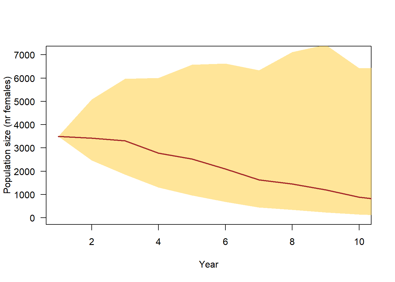
Figure 4.1: 90% simulation range of population trajectories based on current demographic parameter knowledge.
4.4 Sensitivity of the population model to parameter changes
To evaluate the sensitivity of the population trend \(\lambda\) ito alterations in specific parameter values, we used a deterministic matrix model to calculate the population growth rate, determined by the dominant eigenvalue of the Lefkovitch matrix (Caswell 2001; Pastor 2008). We systematically varied one of demographic parameter at a time while keeping the other parameters at their average values, as used for the simulation above. For this sensitivity analysis, we considered females only. We calculated fecundity, the average number of female offspring produced by a female, using the equation \((1-P(non-breeder))*(f_{1st brood} + P(2nd brood)*f_{2nd brood})/2\), where \(P(non-breeder)\) represents the proportion of non-breeders, \(f_{1st brood}\) and \(f_{2nd brood}\) the number of fledglings in the first and second brood and \(P(2nd brood)\) stands for the proportion of females doing a second brood among the breeding females. We assume a sex ratio of 1:1 among the fledglings as it was also the case for the stochastic population model (simulation above).
Even though the units of measurements for different demographic parameters are not directly comparable, we conclude that minor changes in survival, particularly juvenile survival, have a substantial impact on population growth rate. Conversely, altering the average number of nestlings from two to five has only a minor effect on the population growth rate (Figure 4.2). The proportion of non-breeders has a more substantial impact on the population growth compared to the proportion of second broods. However, the question which of the two parameters is the more important driver of population growth, also depends on the variance in the parameters. Data on these parameters are currently being collected.
These findings lead us to conclude that, for predicting future population trends, it is critical to understand how survival is linked to environmental variables. Furthermore, knowing the proportion of non-breeders and the proportion of second broods is more crucial than accurately estimating the average number of fledglings.
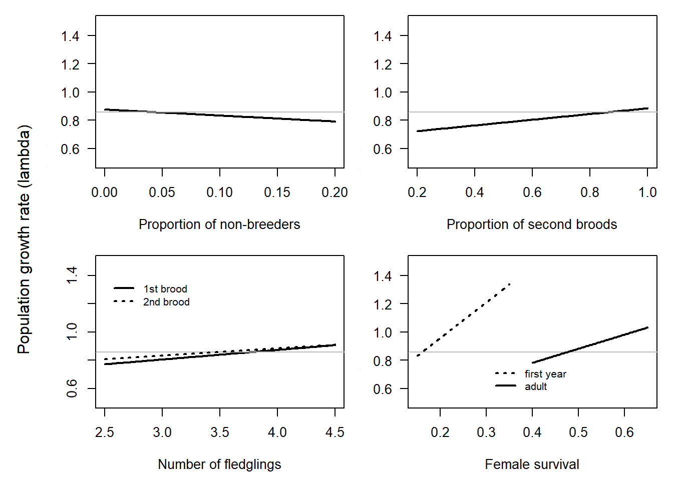
Figure 4.2: Sensitivity of the population growth rate to changes in single demographic parameters deduced from a deterministic matrix model. A single parameter is modified at a time while all others were retained at the values used for the simulation. The scales of the x-axes are chosen so that they span the range of currently plausible seeming average values. The grey horizontal line indicates the population trend for average parameter values.
4.5 For which parameter would additional data improve predicted population trends most?
To determine which information increases precision of the predicted population trajectories the most, we conducted simulations, presuming we exactly knew a specific parameter value. We run separate analyses for 1) the proportions of non-breeders, single and double brooded pairs, 2) the number of fledglings per brood, and 3) survival.
Having precise knowledge of 1) the average number of broods per pair (i.e. the proportions of non-breeders, single and double brooded pairs), and 2) the number of fledglings per brood, it will have similar effects on the precision of the predicted population trends (Figure 4.3). In both cases, the uncertainty of the predicted population size in 10 years is reduced from 140 - 6430 females to ranges of 123 - 5625 females if 1) the average number of broods is exactly known and 108 - 5476 females if 2) the average number of fledglings is exactly known. However, the most pronounced increase in precision of the projected population size occurs when survival is exactly known. In this scenario, the predicted number of females in 10 years ranges between 812 to 2566.
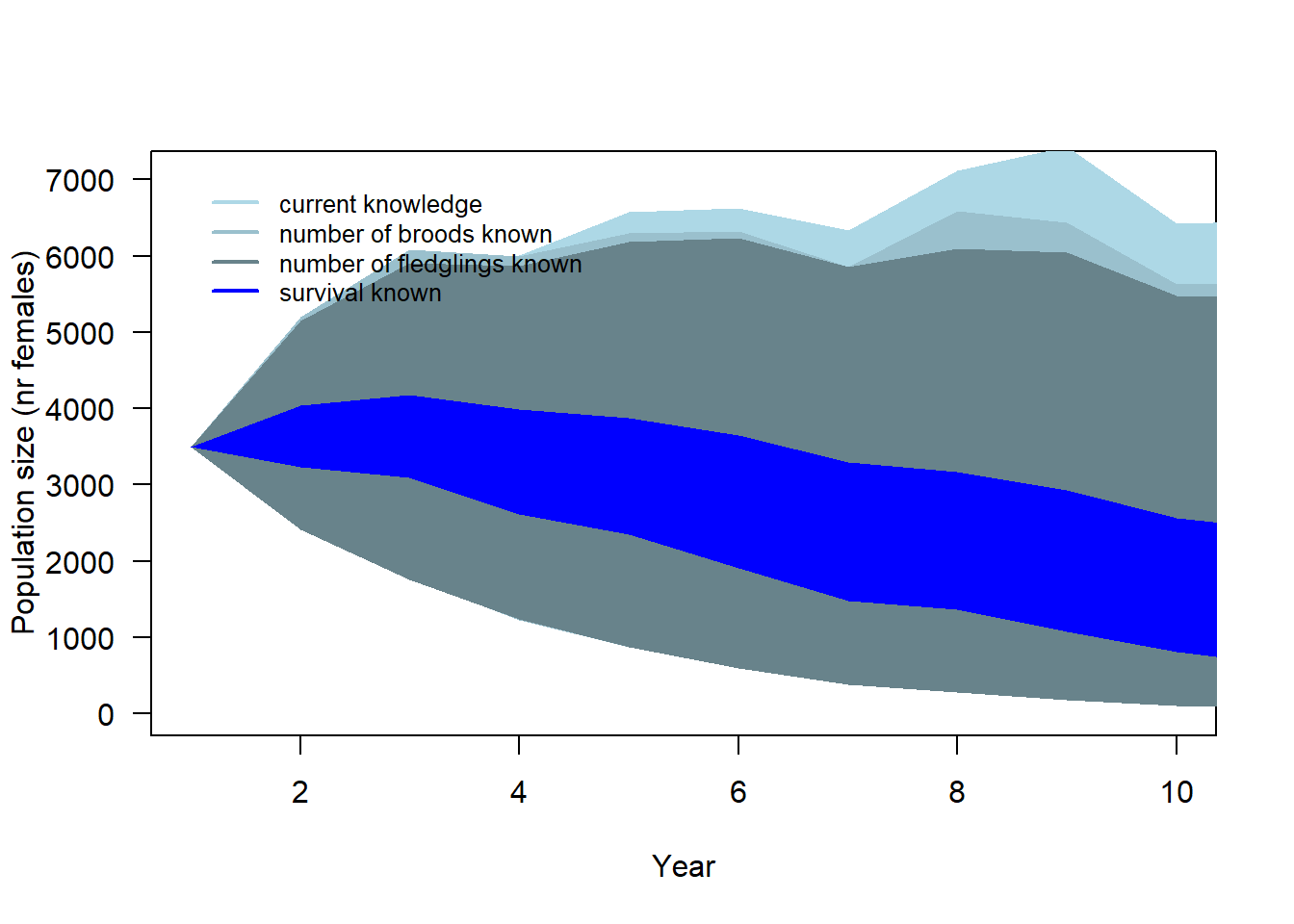
Figure 4.3: 90% simulation range of population trajectories based on current demographic parameters knowledge.